|
Cite as: “R.D. Pascual-Marqui: Discrete, 3D distributed, linear imaging methods of electric neuronal activity. Part 1: exact, zero
error localization. arXiv:0710.3341 [math-ph], 2007-October-17, http://arxiv.org/pdf/0710.3341 ”
Page 10 of 16
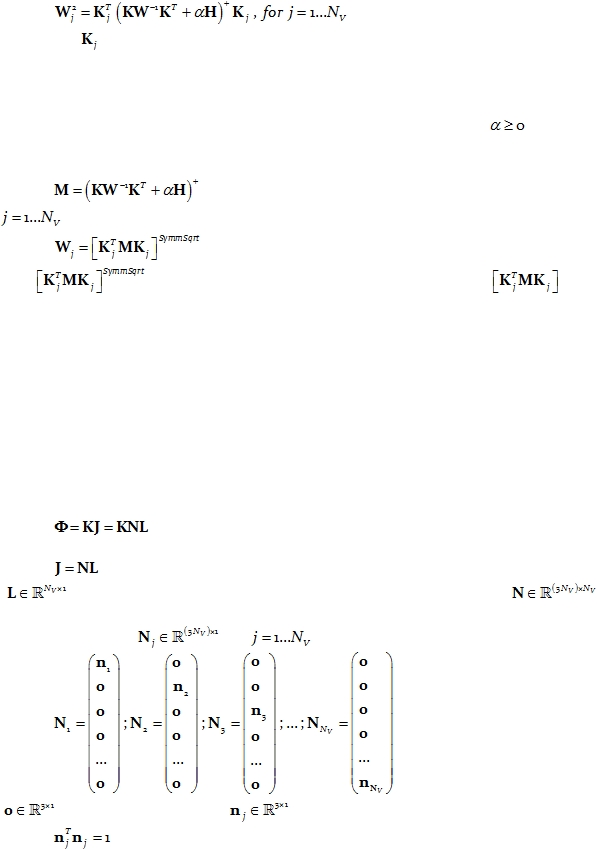
The solution to the problem in Eq. 42 satisfies the following set of matrix equations:
Eq. 43:
where the matrix
is defined in Eq. 7.
The following simple iterative algorithm
(in pseudo-code) converges to the block-
diagonal weights W that solve the problem in Eq. 42 and equivalently satisfies Eq. 43:
1. Given the average reference lead field K and a regularization parameter
, initialize
the block-diagonal weight matrix W as the identity matrix.
2. Set:
Eq. 44:
3. For
do:
Eq. 45:
Comment:
denotes the symmetric square root of the matrix
.
4. Go to step 2 until convergence (negligible changes in W).
Finally, the block-diagonal matrix W produced by this algorithm should be plugged
into the pseudoinverse matrix T
(in Eq. 37). This is denoted as the eLORETA inverse
solution.
7.3.
eLORETA for EEG with known current density vector orientation,
unknown amplitude
The average reference forward EEG equation (Eq. 14) is now written as:
Eq. 46:
with:
Eq. 47:
where
contains the current density amplitudes
at each voxel, and
contains the outward
normal vectors to the cortical surface
at each voxel. Note that the
columns of N, denoted as
for
are:
Eq. 48:
where
is a vector of zeros, and
is the normal vector at the j-th voxel, i.e.:
Eq. 49:
In this section, N is assumed to be known.