|
Cite as: “R.D. Pascual-Marqui: Discrete, 3D distributed, linear imaging methods of electric neuronal activity. Part 1: exact, zero
error localization. arXiv:0710.3341 [math-ph], 2007-October-17, http://arxiv.org/pdf/0710.3341 ”
Page 11 of 16
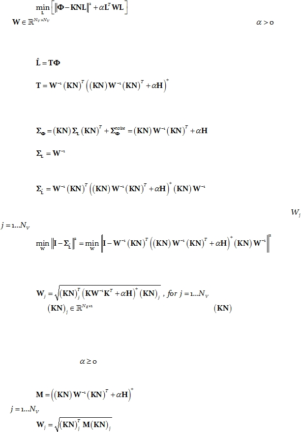
The regularized, weighted minimum norm problem is:
Eq. 50:
where
in this case denotes a given symmetric weight matrix, and
denotes
the regularization parameter.
The solution is linear:
Eq. 51:
with:
Eq. 52:
Following similar lines of reasoning as in the previous section, the covariance matrix
for the electric potential is:
Eq. 53:
where:
Eq. 54:
is the “a priori” covariance matrix for the current density amplitudes L.
In addition, the
covariance matrix for the estimated current density is:
Eq. 55:
When W is restricted to be a diagonal matrix, with the j-th element denoted as
,
for
, then the solution to the problem:
Eq. 56:
produces an inverse solution (Eq. 51 and Eq. 52) with zero localization error.
The solution to the problem in Eq. 56 satisfies the following set of equations:
Eq. 57:
where the vector
corresponds to the j-th column of
.
The following simple iterative algorithm (in pseudo-code) converges to the diagonal
weights W that solve the problem in Eq. 56 and equivalently satisfies Eq. 57:
1. Given the average reference lead field K, the cortical normal vectors N, and a
regularization parameter
, initialize the diagonal weight matrix W
as the identity
matrix.
2. Set:
Eq. 58:
3. For
do:
Eq. 59:
4. Go to step 2 until convergence (negligible changes in W).